properties of quantum mechanics, with no classical equivalent17. This property is, notably, one of the foundations of quantum computing, where one of the key aspects is the possibility of creating states that superimpose two qubits, such as in the state |u⟩ = c₀ |0⟩ + c₁ |1⟩. Such a property is uniquely associated with quantum mechanics and the linear structure that underpins it. It is also important to note that the decomposition (1) is not unique: it is possible to decompose a state over the set of eigenstates associated with different operators (corresponding to dif-ferent physical quantities).
Note that the identification of each weight ck(t) in the decomposition (1) is done by calculating the scalar product of ∣Ψ(t)⟩ with the eigenvector |ak⟩ of the operator Â:
(2)
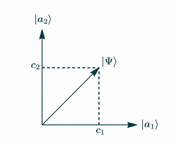
where we have used the orthogonality of the vectors {|an⟩}18. The expression above is nothing more than the generalization, in the abstract space 𝓗, of the projec-tion of a vector from the real space onto the axes of an orthonormal frame (see figure (1) illustrating the projection of a vector in ℝ² onto an orthonormal frame), each coefficient ck representing the “overlap” of the state |Ψ(t)⟩ with the basis vector |ak⟩.
To complete this discussion, it is interesting to consider the case of an observable whose spectrum of values may be continuous, such as the “position” operator 𝑥̂. One writes, in a manner analogous to (1):
(3)
where the summation is replaced by an integral, similarly to (2):
Here, we find, as “coefficients” of the decomposition of |Ψ(t)⟩ over the position eigenstates {|x′⟩}, the wavefunction ψ(x, t) from the “old” quantum mechanics, at the considered point x.
Temporal Evolution: Schrödinger’s Equation
It is assumed that at a given time t0, the system is described by the state vector |ψ0⟩. If no measurement occurs between times t0 and t, the time evolution of the system’s state vector is governed by the following differential equation, known as the Schrödinger equation:
(4)
where ℏ = h/2π, with h being Planck’s constant. The operator Ĥ, called the Hamiltonian, is associated with the energy quantity of the system. Thus, the phys-ical interpretation of equation (4) is that the rate of change of the state vector is
Figure 1 – Pictorial representation of the decompo-sition of a quantum state onto a basis consisting of two orthogonal states |a1⟩ and |a2⟩. Here, a vector from the ℝ² space of two-component real vectors is decom-posed into its projections c1 and c2 onto the «axes» |a1⟩ and |a2⟩, respectively.